
Table of Contents
Introduction
This case study uses HTSanalyzeR2 to perform gene set over-representation analysis, enrichment analysis and enriched subnetwork analyses on a common gene expression profile. Basically, this dataset is from a micro-array experiment on 90 colon cancer patients with GEO number named GSE33113. Using the Colon Cancer Consensus Molecular Subtyping classifier generated by Guinney J et al. in 2015 (Guinney J (2015)), we can easily get the subtype label of each patient. Motivated by the poorest prognosis of CMS4 patients, we want to detect the enriched pathways of CMS4 patients compared to non-CMS4 patients. To this end, first we need to do the differential expression analysis using the most popular R packge ‘limma’ tailored for micro-array data. However, to make this vignette simple enough, we skip to exlpain this step and start from the result gotten by ‘limma’.
1. Hypergeometric test and gene set enrichment analysis
1.1 Prepare the input data
To perform gene set enrichment analysis for single dataset, you must preprare the following inputs:
- a named numeric vector of phenotypes (normally this would be a vector of genes with log2 fold change).
- a list of gene set collections (could be generated by HTSanalyzeR2 or use customized gene sets).
First you need to prepare a named phenotype.
data(GSE33113_limma)
phenotype <- as.vector(GSE33113_limma$logFC)
names(phenotype) <- rownames(GSE33113_limma)
Then, if you want to do hypergeometric test on a list of interested genes simultaneously, you need to define the ‘hits’ as your interested genes. For example, here we define the hits as genes with absolute log2 fold change greater than 1 and adjust p value less than 0.05. In this case, the names of phenotype, namely all the input genes, would be taken as the background gene list to perform hypergeometric test.
Note:In cases if you want to do hypergeometric test with only a list of hits and no phenotype, HTSanalyzeR2 can also realize it. For details please go to Part5: Special usage of HTSanalyzeR2.
## define hits if you want to do hypergeometric test
hits <- rownames(GSE33113_limma[abs(GSE33113_limma$logFC) > 1 & GSE33113_limma$adj.P.Val < 0.05, ])
Then we must define the gene set collections. A gene set collection is a list of gene sets, each of which consists of a group of genes with a similar known function. HTSanalyzeR2 provides facilities which greatly simplify the creation of up-to-date gene set collections including three Gene Ontology terms: Molecular Function (MF), Biological Process (BP), Cellular Component (CC) and KEGG pathways. Gene sets in a comprehensive molecular signatures database, MSigDB(Arthur Liberzon (2011)), for Homo Sapiens and Mus musculus are also provided. Here to simplify the demonstration, we will only use one GO, KEGG and one MSigDB gene set collection. To work properly, you need to choose the right species for your input genes. Besides, these gene set collections must be provided as a named list as below:
## generate gene set collection
GO_MF <- GOGeneSets(species="Hs", ontologies=c("MF"))
PW_KEGG <- KeggGeneSets(species="Hs")
MSig_C2 <- MSigDBGeneSets(collection = "c2", species = "Hs")
## combine all needed gene set collections into a named list for further analysis
ListGSC <- list(GO_MF=GO_MF, PW_KEGG=PW_KEGG, MSig_C2=MSig_C2)
1.2 Initialize and preprocess
An S4 class named ‘GSCA’ is developed to perform hypergeometric test in order to find the gene sets sharing significant overlapping with hits. Gene set enrichment analysis, as described by Subramanian et al. (Subramanian A (2005)), can also be conducted.
To initialize a new ‘GSCA’ object, the previous prepared phenotype and a named list of gene sets collections are needed. In addition, as said before, if you also want to do hypergeometric test, ‘hits’ is needed.
gsca <- GSCA(listOfGeneSetCollections=ListGSC,
             geneList=phenotype, hits=hits)
Then a preprocess step including invalid input data removing, duplication removing by different methods, initial gene identifiers converting to Entrez ID and phenotype ordering needs to be performed to fit for the next analysis. See the help documentation of funciton preprocess for more details.
1.3 Perform analysis
After getting a preprocessed ‘GSCA’ object, you can perform hypergeometric test and gene set enrichment analysis using the function named analyze. This funciton needs an argument called para, which is a list of parameters including:
- pValueCutoff : a single numeric value specifying the cutoff for adjusted pvalues considered significant.
- pAdjustMethod: a single character value specifying the pvalue adjustment method.
- nPermutations: a single numeric value specifying the number of permutations for deriving p-values of GSEA.
- minGeneSetSize: a single numeric value specifying the minimum number of genes shared by a gene set and the background genes, namely the phenotype. Gene sets with fewer than this number are removed from both hypergeometric test and GSEA.
- exponent: a single integer or numeric value used in weighting phenotypes in GSEA, as described by Subramanian et al. (Subramanian A (2005)).
gsca2 <- analyze(gsca1,
                 para=list(pValueCutoff=0.05, pAdjustMethod="BH",
                 nPermutations=100, minGeneSetSize=150,
                 exponent=1),
                 doGSOA = TRUE, doGSEA = TRUE)
In this case study, we only use 100 permutations and set a very large minGeneSetSize just for a fast compilation of this vignette. In real applications, you may want a much smaller threshold (e.g. 10) and more permutations (e.g. 1000) to get a more robust GSEA result.
During the enrichment analysis of gene sets, the function evaluates the statistical significance of the gene set scores by performing a large number of permutations. To perform it more efficiently, our package allows parallel calculation based on the doParallel package. To do this, the user simply needs to register and claim to use multiple cores before running analyze.
## analyze using 4 cores
if (requireNamespace("doParallel", quietly=TRUE)) {
    doParallel::registerDoParallel(cores=4)
} else {
}
gsca2 <- analyze(gsca1,
                 para=list(pValueCutoff=0.05, pAdjustMethod="BH",
                 nPermutations=100, minGeneSetSize=150,
                 exponent=1),
                 doGSOA = TRUE, doGSEA = TRUE)
After analyzing, all the results are stored in slot result and can be easily accessed using a function named getResult. If hypergeometric test and GSEA are both performed, gene sets which are both significant in this two kinds of analysis based on either pvalue or adjusted pvalue can be accessed.
## 1. hypergeometric test result using BP gene sets from GO
head(getResult(gsca2)$HyperGeo.results$GO_MF, 3)
##          Universe Size Gene Set Size Total Hits Expected Hits
## GO:0005509        18865          628        450    14.980122
## GO:0008083        18865          150        450    3.578055
## GO:0042803        18865          751        450    17.914127
##          Observed Hits         Pvalue    Adjusted.Pvalue
## GO:0005509           41  5.887557e-09     4.817155e-08
## GO:0008083           14  1.474862e-05     7.964255e-05
## GO:0042803           31  2.254969e-03     8.335333e-03

## 2. GSEA result using KEGG gene sets
head(getResult(gsca2)$GSEA.results$PW_KEGG, 3)
##          Observed.score       Pvalue     Adjusted.Pvalue
## hsa04022       0.4977871           0                  0
## hsa00230      -0.3699180           0                  0
## hsa05152       0.5278489           0                  0

## 3. result both significant regarding to pvalues in hypergeometric test
##    and GSEA using 'c2' gene sets from MSigDB
head(getResult(gsca2)$Sig.pvals.in.both$MSig_C2, 3)
##                                                    HyperGeo.Pvalue
## TAKEDA_TARGETS_OF_NUP98_HOXA9_FUSION_8D_UP             1.590818e-05
## TONKS_TARGETS_OF_RUNX1_RUNX1T1_FUSION_ERYTHROCYTE_UP   1.590818e-05
## BIDUS_METASTASIS_DN                                    1.039777e-02
##                                                       GSEA.Pvalue
## TAKEDA_TARGETS_OF_NUP98_HOXA9_FUSION_8D_UP                 0
## TONKS_TARGETS_OF_RUNX1_RUNX1T1_FUSION_ERYTHROCYTE_UP       0
## BIDUS_METASTASIS_DN                                        0

## 4. result both significant regarding to adjust pvalues in hypergeometric test
##    and GSEA using 'c2' gene sets from MSigDB
head(getResult(gsca2)$Sig.adj.pvals.in.both$MSig_C2, 3)
##                                                    HyperGeo.Adj.Pvalue
## TAKEDA_TARGETS_OF_NUP98_HOXA9_FUSION_8D_UP             8.372016e-05
## TONKS_TARGETS_OF_RUNX1_RUNX1T1_FUSION_ERYTHROCYTE_UP   8.372016e-05
## BIDUS_METASTASIS_DN                                    3.089480e-02
##                                                       GSEA.Adj.Pvalue
## TAKEDA_TARGETS_OF_NUP98_HOXA9_FUSION_8D_UP                  0
## TONKS_TARGETS_OF_RUNX1_RUNX1T1_FUSION_ERYTHROCYTE_UP        0
## BIDUS_METASTASIS_DN                                         0
In addition, to make the results more understandable, users are highly recommended to annotate the gene sets ID to names by function appendGSTerms. As a result, an additional column named ‘Gene.Set.Term’ would appear.
gsca3 <- appendGSTerms(gsca2, goGSCs=c("GO_MF"),
                       keggGSCs=c("PW_KEGG"),
                       msigdbGSCs = c("MSig_C2"))

head(getResult(gsca3)$GSEA.results$PW_KEGG, 3)
##                        Gene.Set.Term         Observed.score  Pvalue  Adjusted.Pvalue
## hsa04022    cGMP-PKG signaling pathway          0.4977871       0          0
## hsa00230         Purine metabolism             -0.3699180       0          0
## hsa05152 T             uberculosis              0.5278489       0          0
1.4 Summarize results
A summarize method could be performed to get a general summary for an analyzed ‘GSCA’ object including the gene set collections, genelist, hits, parameters for analysis and the summary of result.
summarize(gsca3)
##
## -No of genes in Gene set collections:
##        input above min size
## GO_MF   4150        50
## PW_KEGG 329         38
## MSig_C2 3762        533
##
##
## -No of genes in Gene List:
##            input  valid  duplicate removed converted to entrez
## Gene List  21656  21655              21655              18865
##
##
## -No of hits:
##        input   preprocessed
## Hits    469         450
##
##
## -Parameters for analysis:
##                 minGeneSetSize pValueCutoff pAdjustMethod
## HyperGeo Test        150           0.05          BH
##
##                 minGeneSetSize pValueCutoff pAdjustMethod nPermutations exponent
## GSEA                 150           0.05          BH            100          1
##
##
## -Significant gene sets (adjusted p-value< 0.05 ):
##             GO_MF PW_KEGG MSig_C2
## HyperGeo      7      7       224
## GSEA         22     22       401
## Both          7      7       207
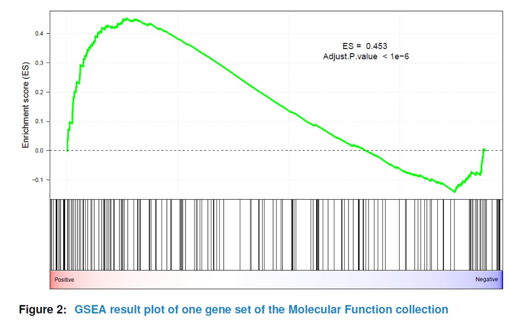
1.5 Plot gene sets
To better view the GSEA result for a single gene set, you can use viewGSEA to plot the positions of the genes of the gene set in the ranked phenotypes and the location of the enrichment score. To this end, you must first get the gene set ID by getTopGeneSets, which can return all or the top significant gene sets from GSEA results. Basically, the user needs to specify the type of results – “HyperGeo.results” or “GSEA.results”, the name(s) of the gene set collection(s) as well as the type of selection– all (by parameter ‘allSig’) or top (by parameter ‘ntop’) significant gene sets.
topGS <- getTopGeneSets(gsca3, resultName="GSEA.results",
                        gscs=c("GO_MF", "PW_KEGG"), allSig=TRUE)
topGS
## $GO_MF
## GO:0008083 GO:0016887 GO:0005125 GO:0004252 GO:0005198
## "GO:0008083" "GO:0016887" "GO:0005125" "GO:0004252" "GO:0005198"
## GO:0003714 GO:0004888 GO:0003779 GO:0001077 GO:0004871
## "GO:0003714" "GO:0004888" "GO:0003779" "GO:0001077" "GO:0004871"
## GO:0004930 GO:0005102 GO:0005509 GO:0042803 GO:0003723
## "GO:0004930" "GO:0005102" "GO:0005509" "GO:0042803" "GO:0003723"
## GO:0005524 GO:0005515 GO:0000287 GO:0003924 GO:0019899
## "GO:0005524" "GO:0005515" "GO:0000287" "GO:0003924" "GO:0019899"
## GO:0000981 GO:0003677
## "GO:0000981" "GO:0003677"
##
## $PW_KEGG
## hsa04022 hsa00230 hsa05152 hsa05016 hsa05202 hsa04360 hsa04062
## "hsa04022" "hsa00230" "hsa05152" "hsa05016" "hsa05202" "hsa04360" "hsa04062"
## hsa04020 hsa04510 hsa05205 hsa04015 hsa04714 hsa04810 hsa04060
## "hsa04020" "hsa04510" "hsa05205" "hsa04015" "hsa04714" "hsa04810" "hsa04060"
## hsa04010 hsa05165 hsa04151 hsa05200 hsa01100 hsa05206 hsa04621
## "hsa04010" "hsa05165" "hsa04151" "hsa05200" "hsa01100" "hsa05206" "hsa04621"
## hsa04014
## "hsa04014"
viewGSEA(gsca3, gscName="GO_MF", gsName=topGS[["GO_MF"]][4])
You can also plot all or the top significant gene sets in batch and store them as png or pdf format into a specified path by using plotGSEA.
plotGSEA(gsca3, gscs=c("GO_MF", "PW_KEGG"), ntop=3, filepath=".")
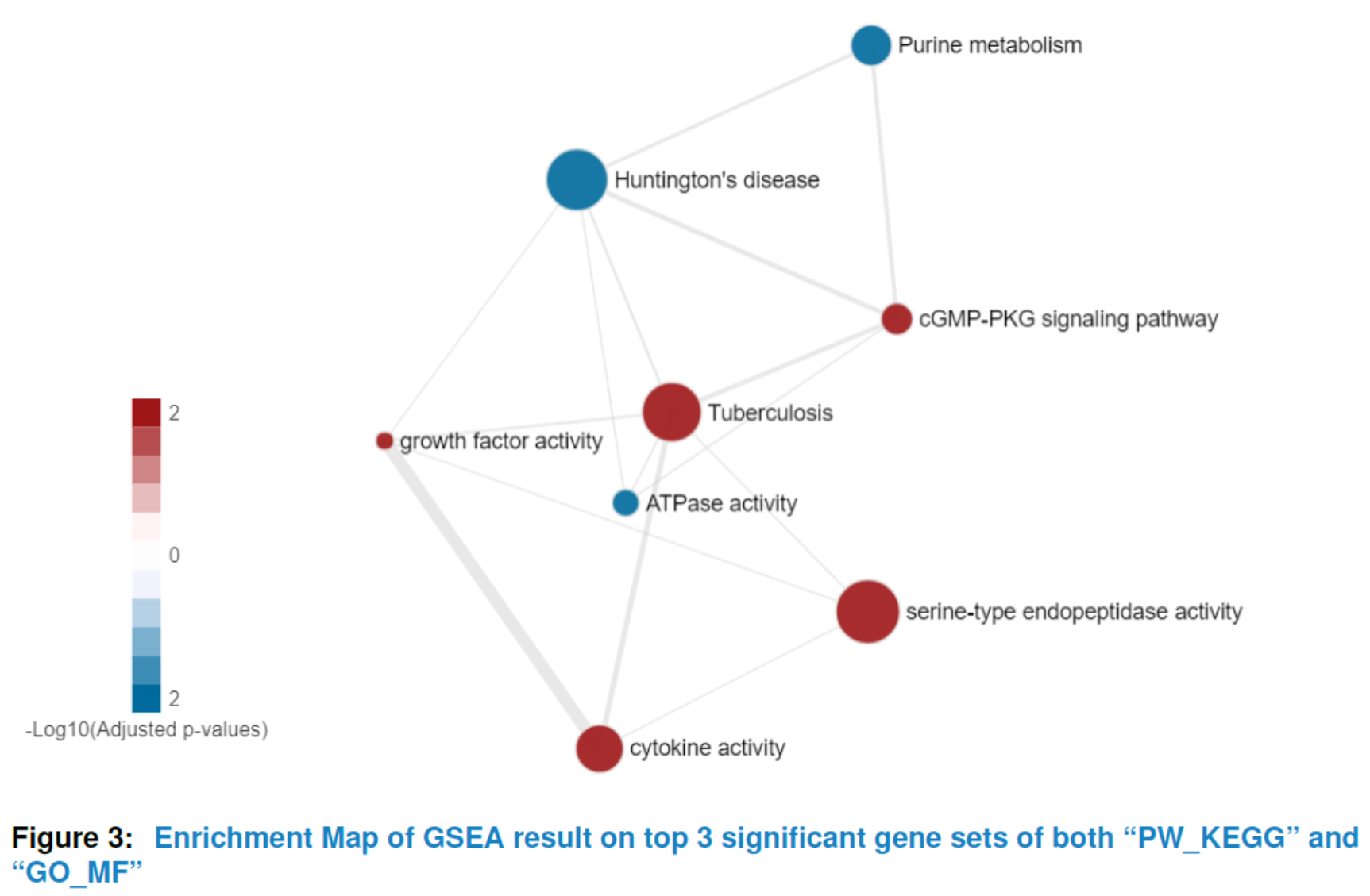
1.6 Enrichment Map
To get a comprehensive view of the hypergeometric test result or GSEA result instead of a list of significant gene sets with no relations, our package provides viewEnrichMap function to draw an enrichment map for better interpretation(Merico D (2010)). More specifically, in the enrichment map, nodes represent significant gene sets sized by the genes it contains and the edge represents the Jaccard similarity coefficient between two gene sets. Nodes color are scaled according to the adjusted pvalues (the darker, the more significant). For hypergeometric test, there is only one color for nodes whereas for GSEA enrichment map, the default color is setted by the sign of enrichment scores (red:+, blue:-). You can also set your favourite format by changing the parameter named ‘options’.
However, users are always highly recommended to use function report to visualize and modify the enrichment map with personal preference in an interactive report, such as different layout, color and size of nodes, types of labels and etc. More details please go to Part4: An interactive Shiny report of results.
## the enrichment map of GSEA result for top 5 significant
## gene sets in 'PW_KEGG' and 'GO_MF'
viewEnrichMap(gsca3, resultName = "GSEA.results",
              gscs=c("PW_KEGG", "GO_MF"),
              allSig = FALSE, gsNameType = "term", ntop = 3)
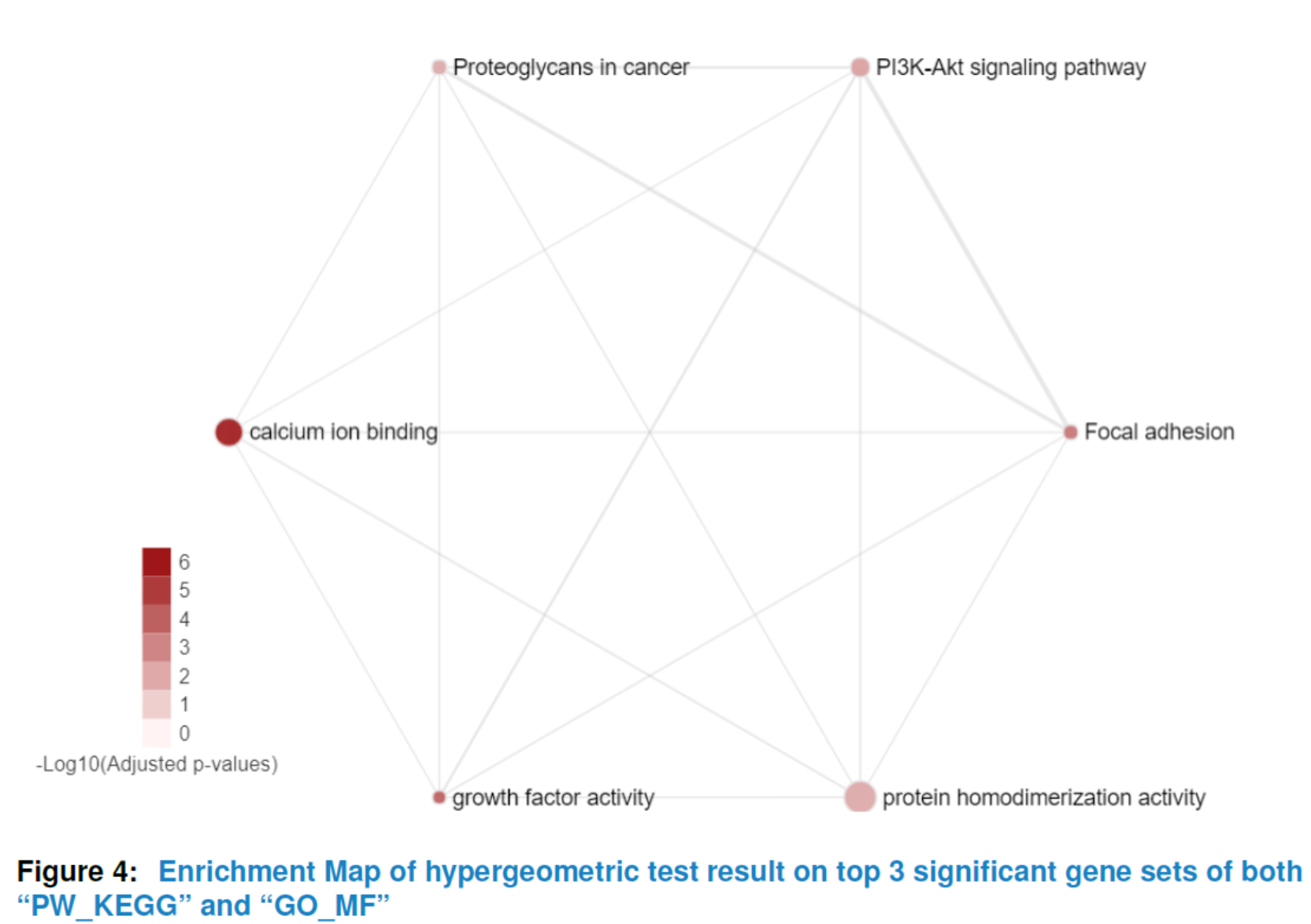
## the enrichment map of hypergeometric test result for
## top 5 significant gene sets in 'PW_KEGG' and 'GO_MF'
viewEnrichMap(gsca3, resultName = "HyperGeo.results",
              gscs=c("PW_KEGG", "GO_MF"),
              allSig = FALSE, gsNameType = "term", ntop = 3)
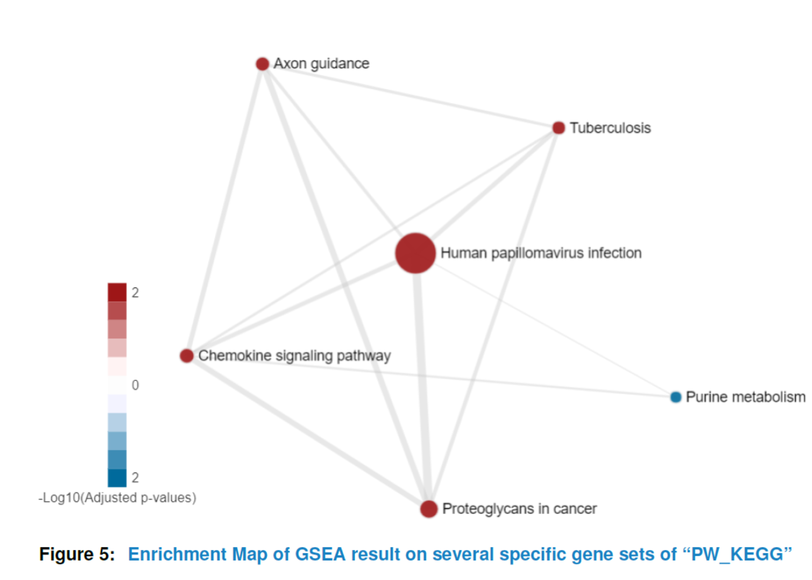
1.7 Enrichment Map with specific gene sets
It is often the case that the enrichment map would be of large size due to the huge number of enriched gene sets. However, you may only be interested in a small part of them. A big size of enrichment map would also be in a mess and lose the information it can offer. In that way, HTSanalyzeR2 provides an interface allowing users to draw the enrichment map on their interested gene sets. More details please see the help documentation of function viewEnrichMap.
## specificGeneset needs to be a subset of all analyzed gene sets
## which can be roughly gotten by:
tmp <- getTopGeneSets(gsca3, resultName = "GSEA.results", gscs=c("PW_KEGG"),
                      ntop = 200, allSig = FALSE)

## In that case, we can define specificGeneset such as below:
PW_KEGG_geneset <- tmp$PW_KEGG[c(2, 3, 6, 7, 10, 18)]

## the name of specificGenesets also needs to match with the names of tmp
specificGeneset <- list("PW_KEGG"=PW_KEGG_geneset)
viewEnrichMap(gsca3, resultName = "GSEA.results", gscs=c("PW_KEGG"),
              allSig = FALSE, gsNameType = "term",
              ntop = NULL, specificGeneset = specificGeneset)
2.Enriched subnetwork analysis
You can also perform subnetwork analysis (Beisser (2010), Dittrich MT (2008)) to extract the subnetwork enriched with nodes which are associated with a significant phenotype using HTSanalyzeR2. The network can either be fetched by our package to download specific species network from BioGRID database or defined by users.
2.1 Prepare input, initialize and preprocess
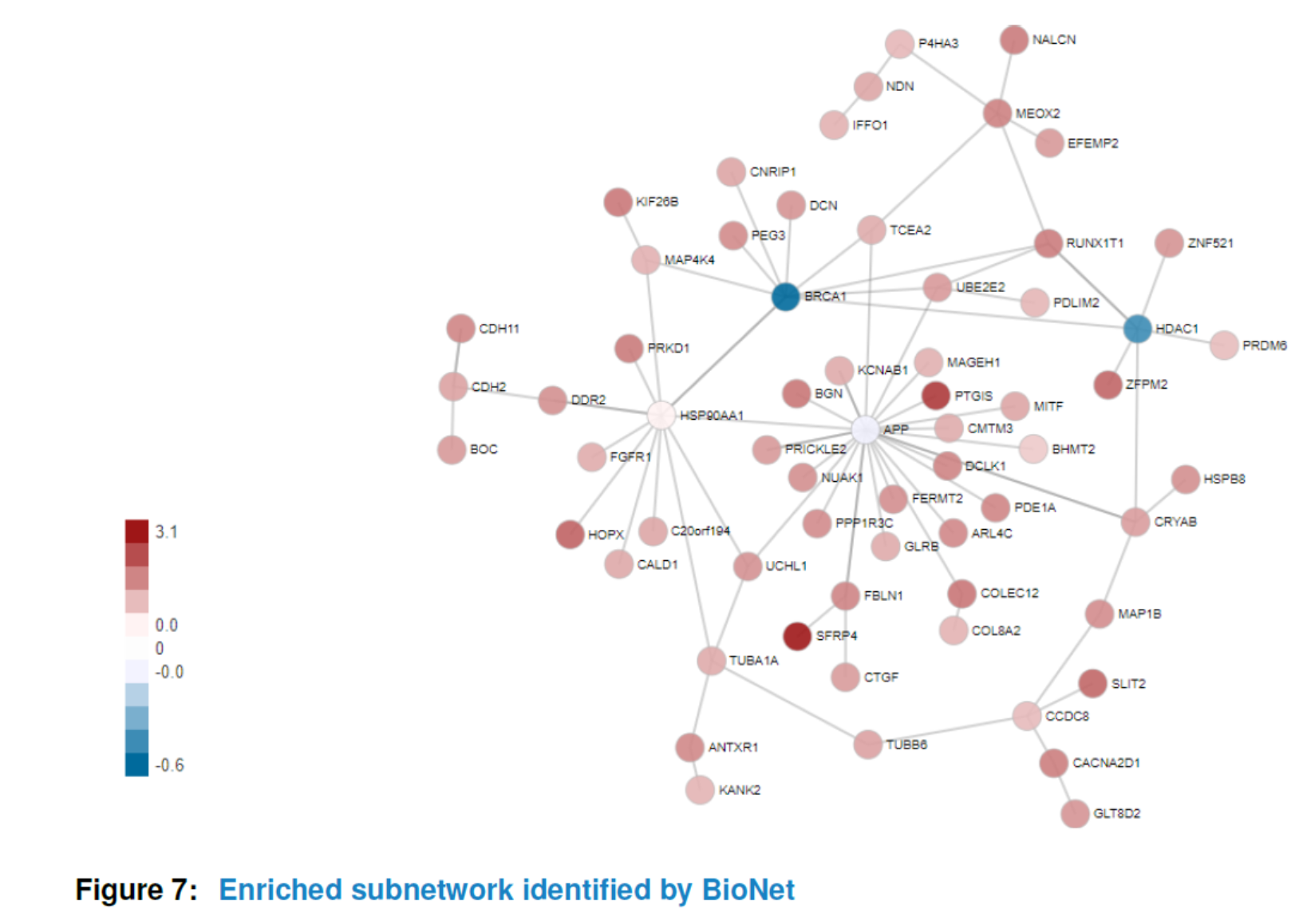
An S4 class named ‘NWA’ is developed to perform subnetwork analysis. To initiate an ‘NWA’ object, you need to prepare a named numeric vector called ‘pvalues’. If phenotypes for genes are also available, they can be inputted in the initialization step and used to highlight nodes with different colors in the identified subnetwork. In that case, the nodes are colored by the sign of phenotypes (red:+, blue:-).
When creating a new object of class ‘NWA’, the user also has the possibility to specify the parameter ‘interactome’ which should be an object of class ‘igraph’. If it is not available, the interactome can also be set up later.
pvalues <- GSE33113_limma$adj.P.Val
names(pvalues) <- rownames(GSE33113_limma)
nwa <- NWA(pvalues=pvalues, phenotypes=phenotype)
The next step is to preprocess the inputs. Similar to ‘GSCA’ class, the function preprocess can conduct invalid input data removing, duplication removing by different methods and initial gene identifiers converting to Entrez ID.
nwa1 <- preprocess(nwa, species="Hs", initialIDs="SYMBOL",
                   keepMultipleMappings=TRUE, duplicateRemoverMethod="max")
Then, you need to create an interactome for the network analysis using method interactome if you have not inputted your own interactome in the initial step. To this end, you can either specify the species and fetch the corresponding network from BioGRID database, or input an interaction matrix if it is in right format: a matrix with a row for each interaction, and at least contains the three columns “InteractorA”, “InteractorB” and “InteractionType”, where the interactors are specified by Entrez ID. For more details please see help(interactome).
Here, we just use interactome to download an interactome from BioGRID, which would meet user’s requirements in most cases.
nwa2 <- interactome(nwa1, species="Hs", genetic=FALSE)
getInteractome(nwa2)
2.2 Perform analysis and view the identified subnetwork
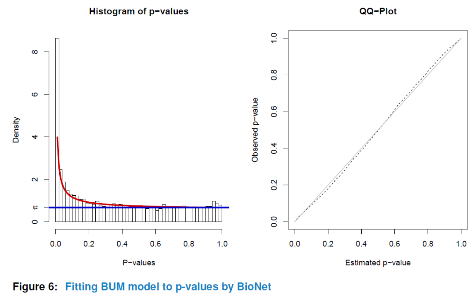
Having preprocessed the input data and created the interactome, the subnetwork analysis could be performed by using the analyze method. This function will plot a figure showing the fitting of the BioNet model to your distribution of pvalues (Beisser (2010)), which is a good way to check the choice of statistics used in this function. The argument fdr of the method analyze is the false discovery rate for BioNet to fit the beta-uniform mixture (BUM) model. The parameters of the fitted model will then be used for the scoring function, which subsequently enables the BioNet package to search the optimal scoring subnetwork. See BioNet for more details (Beisser (2010)).
Here, to simplify this vignette, we set a very strict ‘fdr’ as 1e-06. In practice, you may want to set a less strict one (e.g. 0.01).
nwa3 <- analyze(nwa2, fdr=1e-06, species="Hs")
Similar to ‘GSCA’, you can also view the subnetwork by viewSubNet. Again, for better visualization, modification and downloading, users are highly recommended to view the result in an interactive Shiny report by function report.
viewSubNet(nwa3)
2.3 Summarize results
Like ‘GSCA’, the method summarize could also be used to get a general summary of an analyzed ‘NWA’ object including inputs, interactome, parameters for analysis and the size of identified subnetwork.
summarize(nwa3)
##
## -p-values:
##               input          valid     duplicate removed
##               21656          21655       21655
## converted to entrez in interactome
##               18865          15008
##
##
## -Phenotypes:
##                input          valid    duplicate removed
##                21656          21655      21655
##  converted to entrez  in interactome
##                18865          15008
##
##
## -Interactome:
##                 name    species genetic  node No  edge No
## Interaction dataset Biogrid Hs    FALSE   22439    332134
##
##
## -Parameters for analysis:
##             FDR
## Parameter 1e-06
##
##
## -Subnetwork identified:
##           node No   edge No
## Subnetwork     81   113